using Markdown
using MPSKit, MPSKitModels, TensorKit
using Plots, LaTeXStrings


theme(:wong)
default(fontfamily = "Computer Modern", label = nothing, dpi = 100, framestyle = :box)

1D Bose-Hubbard model

In this tutorial, we will explore the physics of the one-dimensional Bose–Hubbard model using matrix product states. For the most part, we replicate the results presented in Phys. Rev. B 105, 134502, which can be consulted for any statements in this tutorial that are not otherwise cited. The Hamiltonian under study is defined as follows:

where the bosonic creation and annihilation operators satisfy the canonical commutation relations (CCR):

Each lattice site hosts a local Hilbert space corresponding to bosonic occupation states , where  . Since this space is formally infinite-dimensional, numerical simulations typically impose a truncation at some maximum occupation number . Such a treatment is justified since it can be observed that the simulation results quickly converge with the cutoff if the filling fraction is kept sufficiently low.

Within this truncated space, the local creation and annihilation operators are represented by finite-dimensional matrices. For example, with cutoff , the annihilation operator takes the form

and the creation operator is simply its Hermitian conjugate,

The number operator is then given by

Before moving on, notice that the Hamiltonian is uniform and translationally invariant. Typically, such models are studied on a finite chain of sites with periodic boundary conditions, but this introduces finite-size effects that are rather annoying to deal with. In contrast, the MPS framework allows us to work directly in the thermodynamic limit, avoiding such artifacts. We will follow this line of exploration in this tutorial and leave finite systems for another example.

In order to work in the thermodynamic limit, we will have to create an InfiniteMPS. A complete specification of the MPS requires us to define the physical space and the virtual space of the constituent tensors. At this point is it useful to note that MPSKit.jl is powered by TensorKit.jl under the hood and has some very generic interfaces in order to allow imposing symmetries of all kinds. As a result, it is sometimes necessary to be a bit more explicit about what we want to do in terms of the vector spaces involved. In this case, we will not consider any symmetries and simply take the most naive approach of working within the Trivial sector. The physical space is then ℂ^(nmax+1), and the virtual space is ℂ^D where is some integer chosen to be the bond dimension of the MPS, and ℂ is an alias for ComplexSpace (typeset as \bbC). As is increased, one increases the amount of entanglement, i.e, quantum correlations that can be captured by the state.

cutoff, D = 4, 5
initial_state = InfiniteMPS(ℂ^(cutoff + 1), ℂ^D)

1-site InfiniteMPS(ComplexF64, TensorKit.ComplexSpace) with maximal dimension 5:
| ⋮
| ℂ^5
├─[1]─ ℂ^5
│ ℂ^5
| ⋮

This simply initializes a tensor filled with random entries (check out the documentation for other useful constructors). Next, we need the creation and annihilation operators. While we could construct them from scratch, here we will use MPSKitModels.jl instead that has predefined operators and models for most well-known lattice models. In particular, we can use MPSKitModels.a_min to create the bosonic annihilation operator.

a_op = a_min(cutoff = cutoff) # creates a bosonic annihilation operator without any symmetries
display(a_op[])
display((a_op' * a_op)[])

The [] accessor lets us see the underlying array, and indeed the operators are exactly what we require. Similarly, the Bose Hubbard model is also predefined in MPSKitModels.bose_hubbard_model (although we will construct our own variant later on).

hamiltonian = bose_hubbard_model(InfiniteChain(1); cutoff = cutoff, U = 1, mu = 0.5, t = 0.2) # It is not strictly required to pass InfiniteChain() and is only included for clarity; one may instead pass FiniteChain(N) as well

1-site InfiniteMPOHamiltonian(ComplexF64, TensorKit.ComplexSpace) with maximal dimension 4:
| ⋮
| (ℂ^1 ⊞ ℂ^2 ⊞ ℂ^1)
┼─[1]─ ℂ^5
│ (ℂ^1 ⊞ ℂ^2 ⊞ ℂ^1)
| ⋮

This has created the Hamiltonian operator as a matrix product operator (MPO) which is a convenient form to use in conjunction with MPS. Finally, the ground state optimization may be performed with either iDMRG or VUMPS. Both should take similar arguments but it is known that VUMPS is typically more efficient for these systems so we proceed with that.

ground_state, _, _ = find_groundstate(initial_state, hamiltonian, VUMPS(tol = 1.0e-6, verbosity = 2, maxiter = 200))
println("Energy: ", expectation_value(ground_state, hamiltonian))

[ Info: VUMPS init:	obj = +5.514844342897e-01	err = 5.9161e-01
[ Info: VUMPS conv 41:	obj = -6.757777651163e-01	err = 8.1024260014e-07	time = 0.83 sec
Energy: -0.6757777651162759 + 9.071218207774581e-17im

This automatically runs the algorithm until a certain error measure falls below the specified tolerance or the maximum iterations is reached. Let us wrap all this into a convenient function.

function get_ground_state(mu, t, cutoff, D; kwargs...)
    hamiltonian = bose_hubbard_model(InfiniteChain(); cutoff = cutoff, U = 1, mu = mu, t = t)
    state = InfiniteMPS(ℂ^(cutoff + 1), ℂ^D)
    state, _, _ = find_groundstate(state, hamiltonian, VUMPS(; kwargs...))

    return state
end

ground_state = get_ground_state(0.5, 0.01, cutoff, D; tol = 1.0e-6, verbosity = 2, maxiter = 500)

1-site InfiniteMPS(ComplexF64, TensorKit.ComplexSpace) with maximal dimension 5:
| ⋮
| ℂ^5
├─[1]─ ℂ^5
│ ℂ^5
| ⋮

Now that we have the state, we may compute observables using the expectation_value function. It typically expects a Pair, (i1, i2, .., ik) => op where op is a TensorMap or InfiniteMPO acting over k sites. In case of the Hamiltonian, it is not necessary to specify the indices as it spans the whole lattice. We can now plot the correlation function .

plot(map(i -> real.(expectation_value(ground_state, (0, i) => a_op' ⊗ a_op)), 1:50), lw = 2, xlabel = "Site index", ylabel = "Correlation function", yscale = :log10)
hline!([abs2(expectation_value(ground_state, (0,) => a_op))], ls = :dash, c = :black)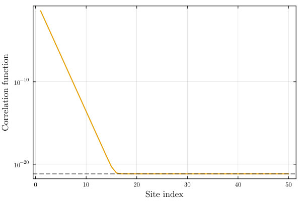

We see that the correlations drop off exponentially, indicating the existence of a gapped Mott insulating phase. Let us now shift our parameters to probe other phases.

ground_state = get_ground_state(0.5, 0.2, cutoff, D; tol = 1.0e-6, verbosity = 2, maxiter = 500)

plot(map(i -> real.(expectation_value(ground_state, (0, i) => a_op' ⊗ a_op)), 1:100), lw = 2, xlabel = "Site index", ylabel = "Correlation function", yscale = :log10, xscale = :log10)
hline!([abs2(expectation_value(ground_state, (0,) => a_op))], ls = :dash, c = :black)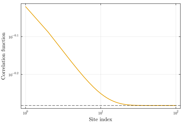

In this case, the correlation function drops off algebraically and eventually saturates as    . This is a signature of long-range order and suggests the existence of a Bose-Einstein condensate. However, this is a bit odd since at zero temperature, the Bose Hubbard model is not expected to break any continuous symmetries ( in this case, corresponding to particle number conservation) due to the Mermin-Wagner theorem. The source of this contradiction lies in the fact that the true 1D superfluid ground state is an extended critical phase exhibiting algebraic decay, however, a finite bond-dimension MPS can only capture exponentially decaying correlations. As a result, the finite bond dimension effectively introduces a length scale into the system in a similar manner as finite-size effects. We can see this clearly by increasing the bond dimension. We also see that the correlation length seems to depend algebraically on the bond dimension as expected from finite-entanglement scaling arguments.

cutoff = 4
Ds = 20:5:50
mu, t = 0.5, 0.2
states = Vector{InfiniteMPS}(undef, length(Ds))

Threads.@threads for idx in eachindex(Ds)
    states[idx] = get_ground_state(mu, t, cutoff, Ds[idx]; tol = 1.0e-7, verbosity = 1, maxiter = 500)
end

npoints = 400
two_point_correlation = zeros(length(Ds), npoints)
a_op = a_min(cutoff = cutoff)

Threads.@threads for idx in eachindex(Ds)
    two_point_correlation[idx, :] .= real.(expectation_value(states[idx], (1, i) => a_op' ⊗ a_op) for i in 1:npoints)
end

p = plot(
    framestyle = :box, ylabel = "Correlation function " * L"\langle a_i^{\dagger}a_j \rangle",
    xlabel = "Distance " * L"|i-j|", xscale = :log10, yscale = :log10,
    xticks = ([10, 100], ["10", "100"]),
    yticks = ([0.25, 0.5, 1.0], ["0.25", "0.5", "1.0"])
)

plot!(
    p, 2:npoints, two_point_correlation[:, 2:end]',
    lab = "D = " .* string.(permutedims(Ds)), lw = 2
)

scatter!(
    p, Ds, correlation_length.(states),
    ylabel = "Correlation length", xlabel = "Bond dimension",
    xscale = :log10, yscale = :log10,
    inset = bbox(0.2, 0.51, 0.25, 0.25),
    subplot = 2,
    xticks = (20:10:50, string.(20:10:50)),
    yticks = ([50, 100], string.([50, 100])),
    xlabelfontsize = 8,
    ylabelfontsize = 8,
    ylims = [20, 130],
    xlims = [15, 60]
)

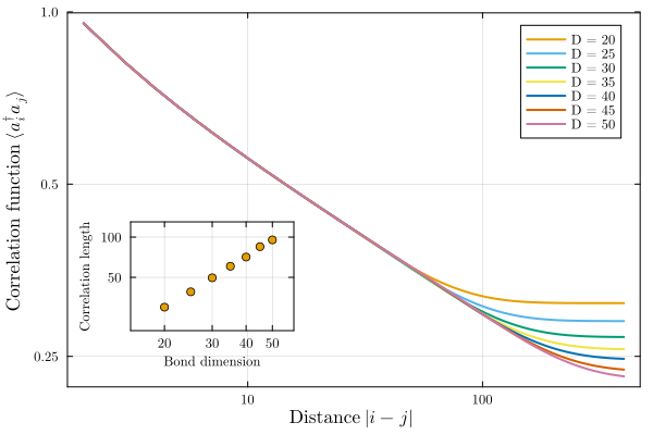
This shows that any finite bond dimension MPS necessarily breaks the symmetry of the system, forming a Bose-Einstein condensate which introduces erroneous long-distance behaviour of correlation functions. In case of finite bond dimension, it is thus reasonable to associate the finite expectation value of the field operator to the 'quasicondensate' density of the system which vanishes as  .

quasicondensate_density = map(state -> abs2(expectation_value(state, (0,) => a_op)), states)

7-element Vector{Float64}:
 0.3097427792977986
 0.2881478005839194
 0.27020015650045337
 0.257127287055965
 0.24685385184650885
 0.23539786293063855
 0.22799664604968056

We may now also visualize the momentum distribution function, which is obtained as the Fourier transform of the single-particle density matrix. Starting from the definition of the momentum occupation operators:

the momentum distribution is

For a translationally invariant system, the correlation depends only on the distance   :

Changing variables (  ) gives

The sum over yields a factor of , which cancels the prefactor, leading to

However, we know that a finite bond dimension MPS introduces a non-zero quasi-condensate density which would give rise to an divergence in the momentum distribution that is not indicative of the true physics of the system. Since we know this contribution vanishes in the infinite bond dimension limit, we instead work with   .

ks = range(-0.05, 0.15, 500)
momentum_distribution = map(
    ((corr, qc),) -> sum(
        2 .* cos.(ks' .* (2:npoints)) .* (corr[2:end] .- qc), dims = 1
    ) .+ (corr[1] .- qc),
    zip(
        eachrow(two_point_correlation),
        quasicondensate_density
    )
)
momentum_distribution = vcat(momentum_distribution...)'
plot(ks, momentum_distribution, lab = "D = " .* string.(permutedims(Ds)), lw = 1.5, xlabel = "Momentum k", ylabel = L"\langle n_k \rangle", ylim = [0, 50])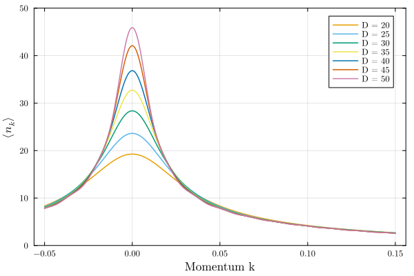

We see that the density seems to peak around  , this time seemingly becoming more prominent as   which seems to suggest again that there is a condensate. However, going by the Penrose-Onsager criterion, the existence of a condensate can be quantified by requiring the leading eigenvalue of the single particle density matrix (i.e,  ) to diverge as in the thermodynamic limit. In this case, since the correlations decay as a power law, there is naturally a divergence at low momenta. But this does not imply the existence of a condensate since the order of divergence is much weaker. However, this does indicate the remnants of some kind of condensation in the 1D model despite the quantum fluctuations, leading to the practical utility of defining the concept of a quasicondensate where there is still a notion of phase coherence over short distances.

What this means for us is that, as far as MPS simulations go, we may still utilize the quasicondensate density as an effective order parameter, although it will be less robust as the bond dimension is increased. Alternatively, we realize that the true phase is characterized as being a superfluid (a concept distinct from Bose-Einstein condensation) and can be identified by a non-zero value of the superfluid stiffness (also known as helicity modulus, ) as defined by Leggett. Upon applying a phase twist to the boundaries of the system, a superfluid phase would suffer an increase in energy whereas an insulating phase would not. In the thermodynamic limit, one could show that the boundary conditions may be considered as periodic and instead uniformly distribute the phase across the chain as  . Concretely, in the limit of  , we have:

In order to find the ground state under these twisted boundary conditions, we must construct our own variant of the Bose-Hubbard Hamiltonian. Typically you would want to take a peek at the source code of MPSKitModels.jl to see how these models are defined and tweak it as per your needs. Here we see that applying twisted boundary conditions is equivalent to adding a prefactor of in front of the hopping amplitudes.

function bose_hubbard_model_twisted_bc(
        elt::Type{<:Number} = ComplexF64, symmetry::Type{<:Sector} = Trivial,
        lattice::AbstractLattice = InfiniteChain(1);
        cutoff::Integer = 5, t = 1.0, U = 1.0, mu = 0.0, phi = 0
    )

    a_pm = a_plusmin(elt, symmetry; cutoff = cutoff)
    a_mp = a_minplus(elt, symmetry; cutoff = cutoff)
    N = a_number(elt, symmetry; cutoff = cutoff)

    interaction_term = N * (N - id(domain(N)))

    return H = @mpoham begin
        sum(nearest_neighbours(lattice)) do (i, j)
            return -t * (exp(1im * phi) * a_pm{i, j} + exp(1im * -phi) * a_mp{i, j})
        end +
            sum(vertices(lattice)) do i
            return U / 2 * interaction_term{i} - mu * N{i}
        end
    end
end

function superfluid_stiffness_profile(t, mu, D, cutoff, ϵ = 1.0e-4, npoints = 11)
    phis = range(-ϵ, ϵ, npoints)
    energies = zeros(length(phis))

    Threads.@threads for idx in eachindex(phis)
        hamiltonian_twisted = bose_hubbard_model_twisted_bc(;
            cutoff = cutoff, t = t, mu = mu, U = 1, phi = phis[idx]
        )
        state = InfiniteMPS(ℂ^(cutoff + 1), ℂ^D)
        state_twisted, _, _ = find_groundstate(
            state, hamiltonian_twisted, VUMPS(; tol = 1.0e-8, verbosity = 0)
        )
        energies[idx] = real(expectation_value(state_twisted, hamiltonian_twisted))
    end

    return plot(phis, energies, lw = 2, xlabel = "Phase twist per site" * L"(\phi)", ylabel = "Ground state energy", title = "t = $t | μ = $mu | D = $D | cutoff = $cutoff")
end

superfluid_stiffness_profile(0.2, 0.3, 5, 4) # superfluid

superfluid_stiffness_profile(0.01, 0.3, 5, 4) # mott insulator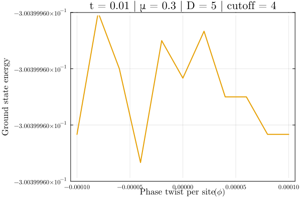

Now that we know what phases to expect, we can plot the phase diagram by scanning over a range of parameters. In general, one could do better by performing a bisection algorithm for each chemical potential to determine the value of the hopping parameter at the transition point, however the 1D Bose-Hubbard model may have two transition points at the same chemical potential which makes this a bit cumbersome to implement robustly. Furthermore, we stick to using the quasi-condensate density as an order parameter since extracting the superfluid density accurately requires a more robust scheme to compute second derivatives which takes us away from the focus of this tutorial.

cutoff, D = 4, 10
mus = range(0, 0.75, 40)
ts = range(0, 0.3, 40)

a_op = a_min(cutoff = cutoff)
order_parameters = zeros(length(ts), length(mus))

Threads.@threads for (i, j) in collect(Iterators.product(eachindex(mus), eachindex(ts)))
    hamiltonian = bose_hubbard_model(InfiniteChain(); cutoff = cutoff, U = 1, mu = mus[i], t = ts[j])
    init_state = InfiniteMPS(ℂ^(cutoff + 1), ℂ^D)
    state, _, _ = find_groundstate(init_state, hamiltonian, VUMPS(; tol = 1.0e-8, verbosity = 0))
    order_parameters[i, j] = abs(expectation_value(state, 0 => a_op))
end

heatmap(ts, mus, order_parameters, xlabel = L"t/U", ylabel = L"\mu/U", title = L"\langle \hat{a}_i \rangle")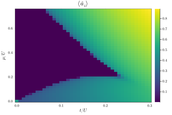

Although the bond dimension here is quite low, we already see the deformation of the Mott insulator lobes to give way to the well known BKT transition that happens at commensurate density. One can go further and estimate the critical exponents using finite-entanglement scaling procedures on the correlation functions, but these may now be performed with ease using what we have learnt in this tutorial.

---

This page was generated using Literate.jl.