using Markdown
using TensorKit
using MPSKit
using MPSKit: infinite_temperature_density_matrix
using MPSKitModels
using QuadGK: quadgk
using SpecialFunctions: ellipe
using Plots
using LinearAlgebra
using BenchmarkFreeFermions

Finite temperature XY model

This example shows how to simulate the finite temperature behavior of the XY model in 1D. Importantly, the Hamiltonian can be diagonalized in terms of fermionic creation and annihilation operators. As a result, many properties have analytical expressions that can be used to verify our results. Here, we use BenchmarkFreeFermions.jl to compare our results.

Here we will consider the anti-ferromagnetic ( ) chain, and restrict ourselves to  .

Parameters

J = 1 / 2
T = ComplexF64
symmetry = U1Irrep

function XY_hamiltonian(
        ::Type{T} = ComplexF64, ::Type{S} = Trivial; J = 1 / 2, N
    ) where {T <: Number, S <: Sector}
    spin = 1 // 2
    term = J * (S_xx(T, S; spin) + S_yy(T, S; spin))
    lattice = isfinite(N) ? FiniteChain(N) : InfiniteChain(1)
    return @mpoham begin
        sum(nearest_neighbours(lattice)) do (i, j)
            return term{i, j}
        end
    end
end

XY_hamiltonian (generic function with 3 methods)

Diagonalization of the Hamiltonian

The Hamiltonian can be diagonalized through a Bogoliubov transformation, leading to the following expression for the ground state energy The Hamiltonian can be diagonalized in terms of fermionic creation and annihilation operators, leading to the following expression in terms of an incomplete elliptic integral of the second kind.

The derivation, via a Jordan-Wigner transformation to free fermions followed by a Bogoliubov rotation, can be found in Lieb, Schultz & Mattis, Ann. Phys. 16, 407 (1961).

function groundstate_energy(J, N)
    isfinite(N) || return -J / π
    T = diagm(1 => J / 2 * ones(N - 1), -1 => J / 2 * ones(N - 1))
    ϵ = SingleParticleSpectrum(T)
    return Energy(ϵ, Inf, 0) / N
end

groundstate_energy (generic function with 1 method)

Exact diagonalization

We can check our results by comparing them to the exact diagonalization of the Hamiltonian.

N_exact = 6
H = open_boundary_conditions(XY_hamiltonian(T, symmetry; J, N = Inf), N_exact)
H_dense = convert(TensorMap, H);
vals = eigvals(H_dense)[one(symmetry)] ./ N_exact
groundstate_energy(J, N_exact)

println("Numerical:\t", minimum(real(vals)))
println("Exact (N=$(N_exact)):\t", groundstate_energy(J, N_exact))
println("Exact (N=Inf):\t", groundstate_energy(J, Inf))

Numerical:	-0.1455816336431223
Exact (N=6):	-0.14558163364312227
Exact (N=Inf):	-0.15915494309189535

Finite MPS

If we wish to increase the system size, we can use the finite MPS representation.

N = 32
H = XY_hamiltonian(T, symmetry; J, N)
D = 64
V_init = symmetry === Trivial ? ℂ^32 : U1Space(i => 10 for i in -1:(1 // 2):1)
psi_init = FiniteMPS(N, physicalspace(H, 1), V_init)
trscheme = truncrank(D)
psi, envs, = find_groundstate(psi_init, H, DMRG2(; trscheme, maxiter = 5));
E_0 = expectation_value(psi, H, envs) / N

println("Numerical:\t", real(E_0))
println("Exact (N=$N):\t", groundstate_energy(J, N))
println("Exact (N=Inf):\t", groundstate_energy(J, Inf))

[ Info: DMRG2   1:	obj = -5.004084869795e+00	err = 9.8826020061e-01	time = 1.04 min
[ Info: DMRG2   2:	obj = -5.004096937587e+00	err = 1.1541480959e-06	time = 0.42 sec
[ Info: DMRG2   3:	obj = -5.004096975044e+00	err = 2.5015824967e-09	time = 0.72 sec
[ Info: DMRG2 conv 4:	obj = -5.004096975044e+00	err = 1.8118839762e-13	time = 1.07 min
Numerical:	-0.15637803047010948
Exact (N=32):	-0.15637803047254015
Exact (N=Inf):	-0.15915494309189535

Finite temperature properties

To go beyond the ground state, we can extract several properties at finite temperature by computing the partition function. This is given by

where   is the inverse temperature.

Given the partition function, we can compute the free energy as

We can also compute observables using

In particular, we can compute the energy as

Finally, the specific heat can be computed as

Luckily, the partition function can be computed analytically for the XY model. The resulting expression is

This expression follows from the same free-fermion diagonalization as the ground-state energy above: each single-particle mode is independently occupied or empty, giving the usual free-fermion partition function (see again Lieb, Schultz & Mattis (1961)).

function partition_function(β::Number, J::Number, N::Number)
    T = diagm(1 => J / 2 * ones(N - 1), -1 => J / 2 * ones(N - 1))
    ϵ = SingleParticleSpectrum(T)
    return LogPartition(ϵ, β, 0) / N
end
function free_energy(β, J, N)
    T = diagm(1 => J / 2 * ones(N - 1), -1 => J / 2 * ones(N - 1))
    ϵ = SingleParticleSpectrum(T)
    return FreeEnergy(ϵ, β, 0) / N
end

βs = 0.0:0.2:8.0

Z_analytic = partition_function.(βs, J, N);
F_analytic = free_energy.(βs, J, N);

MPO approach

We can numerically compute the partition function by explicitly computing the trace of the time-evolution operator. To that end, we first need to build the time-evolution operator , and then compute its trace.

In order to build the time-evolution operator, we can repurpose the make_time_mpo function, which constructs the time-evolution operator for the ground state. However, since we are interested in , instead of , we work with   . In particular, we can approximate the exponential using a Taylor series through the TaylorCluster algorithm.

expansion_orders = 1:3

function logpartition_taylor(β, H; expansion_order)
    dτ = im * β
    expH = make_time_mpo(H, dτ, TaylorCluster(; N = expansion_order))
    return log(real(tr(expH))) / length(H)
end

Z_taylor = map(Iterators.product(βs, expansion_orders)) do (β, expansion_order)
    @info "Computing β = $β at order $expansion_order"
    return logpartition_taylor(β, H; expansion_order)
end
F_taylor = -(1 ./ βs) .* Z_taylor

p_taylor = let
    labels = reshape(
        map(expansion_orders) do N
            return "Taylor N=$N"
        end, 1, :
    )
    p1 = plot(
        βs, Z_analytic; label = "analytic", title = "Partition function",
        xlabel = "β", ylabel = "Z(β)"
    )
    plot!(p1, βs, Z_taylor; label = labels)
    p2 = plot(
        βs, F_analytic; label = "analytic", title = "Free energy",
        xlabel = "β", ylabel = "F(β)"
    )
    plot!(p2, βs, F_taylor; label = labels)
    plot(p1, p2)
end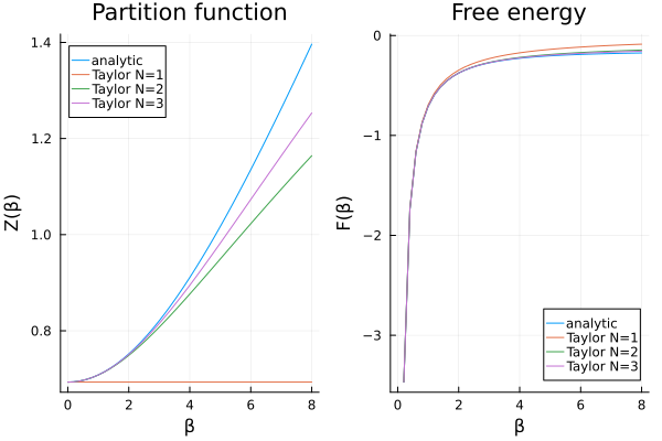

Some observations:

• The first order approximation fails to capture the behavior of the partition function.

• The higher order approximations are in good agreement with the analytical result, as long as is not too large.

• The computational cost of the approximations does not depend on , but on the order of the approximation.

To address the first point, we can have a look at the particular form of the time-evolution operator. Here we see that for this particular Hamiltonian, all the terms with factors are either zero or have trace zero. As a result, the trace of the time-evolution operator is equal to the trace of the identity, hence the result is always .

Therefore, we will exclude the first order approximation from now on. Zooming in on the differences with the analytical result, we find:

expansion_orders = 2:3
Z_taylor = Z_taylor[:, 2:end]
F_taylor = F_taylor[:, 2:end]

p_taylor_diff = let
    labels = reshape(
        map(expansion_orders) do N
            return "Taylor N=$N"
        end, 1, :
    )
    p1 = plot(
        βs, abs.(Z_taylor .- Z_analytic);
        label = labels, title = "Partition function error",
        xlabel = "β", ylabel = "ΔZ(β)", legend = :topleft
    )
    p2 = plot(
        βs, abs.(F_taylor .- F_analytic); label = labels,
        xlabel = "β", ylabel = "ΔF(β)", title = "Free energy error", legend = :topleft
    )
    plot(p1, p2)
end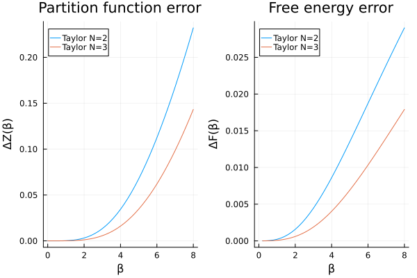

We can now clearly see that, somewhat unsurprisingly, the error increases the larger becomes. Given that we are computing Taylor expansions around  , this is to be expected.

However, there is a trick we can use to improve our results slightly. To that end, we first rewrite the partition function as

In other words, we can compute the partition function at by computing the overlap of two states evolved for , as long as the Hamiltonian is Hermitian. Otherwise, we could still use the same trick, but we would have to compute the evolved states twice, once for and once for .

double_logpartition(ρ₁, ρ₂ = ρ₁) = log(real(dot(ρ₁, ρ₂))) / length(ρ₁)

function logpartition_taylor2(β, H; expansion_order)
    dτ = im * β / 2
    expH = make_time_mpo(H, dτ, TaylorCluster(; N = expansion_order))
    return double_logpartition(expH)
end

Z_taylor2 = map(Iterators.product(βs, expansion_orders)) do (β, expansion_order)
    @info "Computing β = $β at order $expansion_order"
    return logpartition_taylor2(β, H; expansion_order)
end
F_taylor2 = -(1 ./ βs) .* Z_taylor2

p_taylor2_diff = let
    labels = reshape(
        map(expansion_orders[2:end]) do N
            return "Taylor N=$N"
        end, 1, :
    )
    p1 = plot(
        βs, abs.(Z_taylor2 .- Z_analytic);
        label = labels, title = "Partition function error",
        xlabel = "β", ylabel = "ΔZ(β)", legend = :topleft
    )
    p2 = plot(
        βs, abs.(F_taylor2 .- F_analytic); label = labels,
        xlabel = "β", ylabel = "ΔF(β)", title = "Free energy error", legend = :topleft
    )
    plot(p1, p2)
end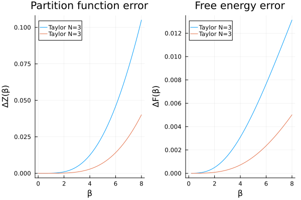

MPO multiplication approach (linear)

While the Taylor series approach is useful, we can only push that so far, since we are always expanding around  . However, inspired by the trick we used to improve the results, we can use MPO multiplication techniques to compute partition functions at larger . In particular, we can implement the following algorithm to scan over a linear range of values.

Multiplying two MPOs exactly would lead to an exponential growth in bond dimensions, but we can make use of standard MPS techniques to keep the bond dimensions under control. To achieve this, we can reinterpret the density matrix as an MPS with two physical indices. Then, we have some control over the approximations we make by tuning the maximal bond dimension.

Here, we swich to a logarithmic scale for the errors to better illustrate the results.

Warning

Using MPS techniques to approximate the multiplication of density matrices does not necessarily inherit all of the nice properties of approximating MPS. In particular, the truncation of the MPO is now happening in the Frobenius norm, rather than the operator norm. While for small truncations this might still work, this is not guaranteed to be the case for larger truncations. As a result, the truncated object might not be positive semidefinite, spoiling its interpretation as a density matrix.

Z_mpo_mul = zeros(length(βs))
D_max = 64

# first iteration: start from high order Taylor expansion
ρ₀ = make_time_mpo(H, im * βs[2] / 2, TaylorCluster(; N = 3))
Z_mpo_mul[1] = Z_taylor[1]
Z_mpo_mul[2] = double_logpartition(ρ₀)

# subsequent iterations: multiply by ρ₀
ρ_mps = convert(FiniteMPS, ρ₀)
for i in 3:length(βs)
    global ρ_mps
    @info "Computing β = $(βs[i])"
    ρ_mps, = approximate(
        ρ_mps, (ρ₀, ρ_mps), DMRG2(; trscheme = truncrank(D_max), maxiter = 10)
    )
    Z_mpo_mul[i] = double_logpartition(ρ_mps)
end
F_mpo_mul = -(1 ./ βs) .* Z_mpo_mul

p_mpo_mul_diff = let
    labels = reshape(
        map(expansion_orders) do N
            return "Taylor N=$N"
        end, 1, :
    )
    p1 = plot(
        βs, abs.(Z_taylor2 .- Z_analytic);
        label = labels, title = "Partition function error",
        xlabel = "β", ylabel = "ΔZ(β)", legend = :bottomright, yscale = :log10
    )
    plot!(
        p1, βs, abs.(Z_mpo_mul .- Z_analytic);
        label = "MPO multiplication"
    )
    p2 = plot(
        βs, abs.(F_taylor2 .- F_analytic); label = labels,
        xlabel = "β", ylabel = "ΔF(β)", title = "Free energy error", legend = nothing,
        yscale = :log10
    )
    plot!(
        p2, βs, abs.(F_mpo_mul .- F_analytic);
        label = "MPO multiplication"
    )
    plot(p1, p2)
end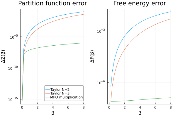

This approach clearly improves the accuracy of the results, indicating that we can indeed compute partition functions at larger values. However, the computational cost of this approach (at fixed maximal bond dimension) is now linear in , since we need to compute the partition function at each value. Often, this is fine, since we are typically interested in a range of values, rather than a single one. However, to really push this to larger values, this can still turn out to be a bottleneck.

We also have to be careful with the accuracy of our results. In particular, the error in the partition function will accumulate over the iterations, which might turn the results into garbage. Typically, the entanglement entropy of the density matrix is a good measure of the required bond dimension, and we can use this to tune the maximal bond dimension.

Apart from the bond dimension, we have two other parameters to tune: the accuracy of the initial density matrix, and the size of the step. The accuracy of the initial density matrix can be improved by increasing the order of the Taylor expansion, but this will result in a larger MPO bond dimension. On the other hand, if we improve the accuracy of the initial density matrix, we could also increase the step size, which would reduce the number of iterations required to reach a certain value. Keeping these parameters in balance is necessary to obtain accurate results, and this might require some trial and error.

MPO multiplication approach (exponential)

If we wish to push the results to even larger values, we can note that taking linear steps in is not the only option. To that end, we can use another trick to scan over an exponential range of values: exponentiating by squaring. In particular, we note that computing for integer (large) can typically be done more efficiently than computing    . To do so, we note that multiplication is associative, and regroup the factors in such a way that we can compute the result in a logarithmic number of steps. Here, we assume   for some integer , and note that this could be generalized to any by decomposing into a sum of powers of . Then, we can write

In other words, we can scan a range of exponentially increasing values by squaring the density matrix at each step.

βs_exp = 2.0 .^ (-3:3)
Z_analytic_exp = partition_function.(βs_exp, J, N)
F_analytic_exp = free_energy.(βs_exp, J, N)

Z_mpo_mul_exp = zeros(length(βs_exp))

# first iteration: start from high order Taylor expansion
ρ₀ = make_time_mpo(H, im * first(βs_exp) / 2, TaylorCluster(; N = 3))
Z_mpo_mul_exp[1] = double_logpartition(ρ₀)

# subsequent iterations: square
ρ = ρ₀
ρ_mps = convert(FiniteMPS, ρ₀)
for i in 2:length(βs_exp)
    global ρ_mps, ρ
    @info "Computing β = $(βs_exp[i])"
    ρ_mps, = approximate(
        ρ_mps, (ρ, ρ_mps), DMRG2(; trscheme = truncrank(D_max), maxiter = 10)
    )
    Z_mpo_mul_exp[i] = double_logpartition(ρ_mps)
    ρ = convert(FiniteMPO, ρ_mps)
end
F_mpo_mul_exp = -(1 ./ βs_exp) .* Z_mpo_mul_exp

p_mpo_mul_exp_diff = let
    labels = reshape(
        map(expansion_orders[2:end]) do N
            return "Taylor N=$N"
        end, 1, :
    )
    p1 = plot(
        βs, abs.(Z_taylor2 .- Z_analytic);
        label = labels, title = "Partition function error", xlabel = "β", ylabel = "ΔZ(β)",
        legend = :bottomright, yscale = :log10
    )
    plot!(p1, βs, abs.(Z_mpo_mul .- Z_analytic); label = "MPO multiplication")
    plot!(p1, βs_exp, abs.(Z_mpo_mul_exp .- Z_analytic_exp); label = "MPO multiplication exp")

    p2 = plot(
        βs, abs.(F_taylor2 .- F_analytic); label = labels, xlabel = "β", ylabel = "ΔF(β)",
        title = "Free energy error", legend = nothing, yscale = :log10
    )
    plot!(p2, βs, abs.(F_mpo_mul .- F_analytic); label = "MPO multiplication")
    plot!(p2, βs_exp, abs.(F_mpo_mul_exp .- F_analytic_exp); label = "MPO multiplication exp")
    plot(p1, p2)
end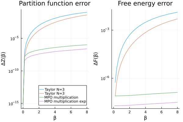

Clearly, the exponential approach allows us to reach larger values much quicker, but there is again a trade-off. Since the size of the steps are increasing, we need to be more careful with the accuracy of our approximations.

Warning

Again, using MPS techniques to approximate the multiplication of density matrices might lead to unphysical truncated density matrices. Increasing the stepsize could make this happen sooner, so we need to be careful with the maximal bond dimension.

Time evolution approach

Finally, we can also note that the partition function is characterized by the following differential equation:

In other words, we can compute the partition function at by evolving the partition function at for a time   .

The starting point for this approach could be either achieved through one of the techniques we have already discussed, but we can also start from the infinite temperature state directly. In particular, this state is given by the identity MPO, and we can evolve this state to compute the partition function at any value.

Z_tdvp = zeros(length(βs))

# first iteration: start from infinite temperature state
ρ₀ = infinite_temperature_density_matrix(H)
Z_tdvp[1] = double_logpartition(ρ₀)

# subsequent iterations: evolve by H
ρ_mps = convert(FiniteMPS, ρ₀)
for i in 2:length(βs)
    global ρ_mps
    @info "Computing β = $(βs[i])"
    ρ_mps, = timestep(
        ρ_mps, H, βs[i - 1] / 2, -im * (βs[i] - βs[i - 1]) / 2,
        TDVP2(; trscheme = truncrank(64))
    )
    Z_tdvp[i] = double_logpartition(ρ_mps)
end
F_tdvp = -(1 ./ βs) .* Z_tdvp

p_mpo_mul_diff = let
    labels = reshape(
        map(expansion_orders) do N
            return "Taylor N=$N"
        end, 1, :
    )
    p1 = plot(
        βs, abs.(Z_taylor2 .- Z_analytic); label = labels,
        title = "Partition function error", xlabel = "β", ylabel = "ΔZ(β)",
        legend = :bottomright, yscale = :log10
    )
    plot!(p1, βs, abs.(Z_mpo_mul .- Z_analytic); label = "MPO multiplication")
    plot!(p1, βs_exp, abs.(Z_mpo_mul_exp .- Z_analytic_exp); label = "MPO multiplication exp")
    plot!(p1, βs, abs.(Z_tdvp .- Z_analytic); label = "TDVP")

    p2 = plot(
        βs, abs.(F_taylor2 .- F_analytic); label = labels, xlabel = "β", ylabel = "ΔF(β)",
        title = "Free energy error", legend = nothing, yscale = :log10
    )
    plot!(p2, βs, abs.(F_mpo_mul .- F_analytic); label = "MPO multiplication")
    plot!(p2, βs_exp, abs.(F_mpo_mul_exp .- F_analytic_exp); label = "MPO multiplication exp")
    plot!(p2, βs, abs.(F_tdvp .- F_analytic); label = "TDVP")

    plot(p1, p2)
end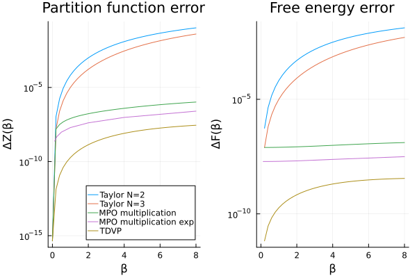

Note

We could further improve the accuracy of the TDVP approach by evolving with    , rather than   which is the current implementation. This is known to improve the stability of the positive semidefinite property of the density matrix, and could lead to more accurate results.

---

This page was generated using Literate.jl.