The transverse-field Ising model: a complete ground-state study

This example is the bridge from the introductory tutorials into the research-grade gallery. If you have worked through Your first ground state and The thermodynamic limit you already know every individual tool used here; the goal now is to assemble them into one coherent case study of a genuine quantum phase transition.

We use the same transverse-field Ising model (TFIM) as the tutorials, on a chain of spin-1/2 sites:

where the first sum runs over neighbouring pairs, sets the energy scale, and the dimensionless field tunes the competition between the interaction and the transverse field. The model has a quantum critical point at  .

Rather than looking at a single field value, we will scan across the transition and diagnose it three independent ways, comparing a finite chain against a calculation performed directly in the thermodynamic limit:

1. the order parameter , computed both for a finite chain and for an infinite chain, in one figure;

2. the entanglement entropy of the infinite state;

3. the correlation length of the infinite state.

All three should point at the same place — that agreement is the payoff.

We take the model and lattice from MPSKitModels, the tensor backend from TensorKit, and Plots for the figures. The Pauli operators σᶻ, σˣ are re-exported by MPSKitModels.

using MPSKit, MPSKitModels, TensorKit, Plots

Shared parameters

We fix a finite chain length L, a bond dimension D (the accuracy knob, see Controlling bond dimension), and the set of field values to scan. D is kept modest so the whole page runs in a couple of minutes; increasing it sharpens the infinite-state diagnostics below (the finite-chain curve responds to D in a less obvious way, as we will see).

L = 16
D = 8
g_values = 0.1:0.1:2.0

0.1:0.1:2.0

1. Finite versus infinite magnetization

We compute the order parameter two ways at every field value.

For the finite calculation we use an open chain of L sites, exactly as in the tutorial, and optimize with DMRG. We average over the sites and take the absolute value: the exact finite-L ground state is symmetric, but DMRG lands on one of the two symmetry-broken states with an arbitrary sign (see the discussion in Your first ground state).

ψ₀_finite = FiniteMPS(L, ℂ^2, ℂ^D)
M_finite = map(g_values) do g
    H = transverse_field_ising(FiniteChain(L); g = g)
    ψ, = find_groundstate(ψ₀_finite, H, DMRG(; verbosity = 0))
    return abs(sum(expectation_value(ψ, i => σᶻ()) for i in 1:L)) / L
end;

For the infinite calculation we drop the lattice argument to build the Hamiltonian on the infinite chain, use an InfiniteMPS, and optimize with VUMPS. We keep every optimized infinite state, because we will reuse them for the entropy and correlation-length diagnostics below.

ψ₀_infinite = InfiniteMPS(ℂ^2, ℂ^D)
states_infinite = map(g_values) do g
    H = transverse_field_ising(; g = g)
    ψ, = find_groundstate(ψ₀_infinite, H, VUMPS(; verbosity = 0))
    return ψ
end;

The order parameter of a translation-invariant state is just on a single site of the unit cell; we again take the absolute value, because on the ordered side the infinite state settles into one of the two symmetry-broken ground states (see The thermodynamic limit).

M_infinite = [abs(expectation_value(ψ, 1 => σᶻ())) for ψ in states_infinite];

Plotting both curves in a single figure lets us compare them directly.

p_magnetization = plot(;
    xlabel = "g", ylabel = "|⟨σᶻ⟩|", title = "TFIM order parameter", legend = :bottomleft
)
scatter!(p_magnetization, g_values, M_finite; label = "finite chain, L = $L, D = $D")
scatter!(p_magnetization, g_values, M_infinite; label = "infinite, D = $D")
vline!(p_magnetization, [1.0]; color = "gray", linestyle = :dash, label = "g = 1")
p_magnetization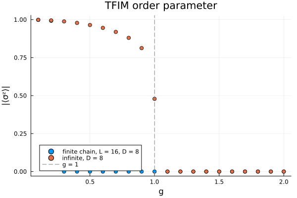

Both calculations agree deep in either phase, but near the transition they tell very different stories. The infinite curve stays on its ordered branch essentially up to g = 1 and then collapses: it locates the critical point cleanly. The finite-chain curve instead drops to zero far earlier — at this L and D the variational optimum on the open chain switches from the symmetry-broken branch to the exactly symmetric ground state, whose magnetization vanishes. Where that switch happens is set by L and D, not by the physics; the same sweep at D = 4 in Your first ground state puts it elsewhere. That is the real lesson of this panel: the finite-chain order parameter is dominated by which state the algorithm selects, while the calculation performed directly in the thermodynamic limit pins the transition at g = 1.

2. Entanglement entropy across the transition

Entanglement is a hallmark of criticality: it is bounded away from the critical point but grows sharply as we approach it. For an InfiniteMPS, entropy returns the von Neumann entanglement entropy per bond, one value for each site of the unit cell. Our unit cell has a single site, so we take the one entry with only.

S_infinite = [real(only(entropy(ψ))) for ψ in states_infinite]
p_entropy = scatter(
    g_values, S_infinite;
    xlabel = "g", ylabel = "entanglement entropy S", title = "TFIM entanglement entropy",
    legend = false
)
vline!(p_entropy, [1.0]; color = "gray", linestyle = :dash)
p_entropy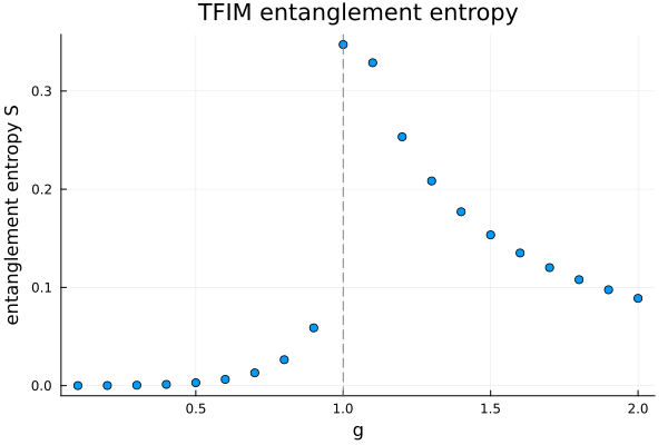

The entropy peaks near g = 1. That peak is the entanglement signature of the phase transition: at criticality correlations become long-ranged and the ground state is at its most entangled, whereas deep in either phase the state is closer to a simple product and the entropy is small.

3. Correlation length across the transition

The correlation_length measures how far apart two spins can still influence each other; it is extracted from the transfer-matrix spectrum of the uniform infinite state and has no finite-chain analogue. It grows toward criticality, so we plot it on a logarithmic vertical axis to make the growth visible.

ξ_infinite = [correlation_length(ψ) for ψ in states_infinite]
p_xi = scatter(
    g_values, ξ_infinite;
    xlabel = "g", ylabel = "correlation length ξ", yscale = :log10,
    title = "TFIM correlation length", legend = false
)
vline!(p_xi, [1.0]; color = "gray", linestyle = :dash)
p_xi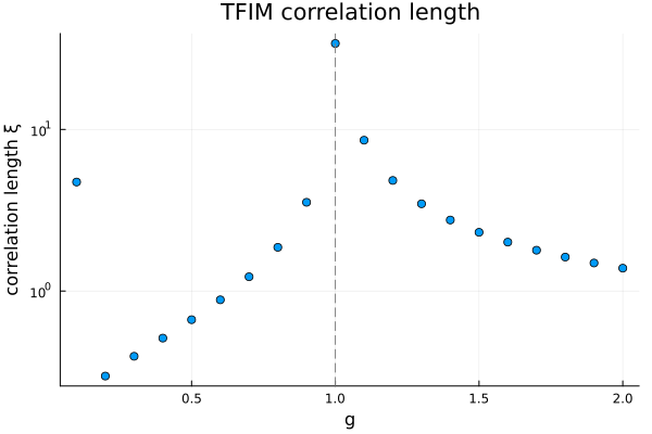

The correlation length peaks near g = 1 as well. At a genuine critical point it would diverge, but a finite bond dimension D can only capture correlations out to a finite range, so what we measure is large-but-capped rather than infinite — the peak grows and sharpens as D is increased.

What you now have

Three independent diagnostics — the order parameter, the entanglement entropy, and the correlation length — all locate the transition of the transverse-field Ising model near g = 1, and the finite-versus-infinite comparison shows concretely why the thermodynamic limit is the right place to measure it.

From here the gallery goes further. The Ising CFT example extracts the momentum-resolved excitation spectrum right at criticality and matches it to the predictions of conformal field theory, turning the "there is a critical point near g = 1" of this page into a quantitative fingerprint of which critical theory it is. Every curve on this page also sharpens if you rerun it at a larger bond dimension D.

---

This page was generated using Literate.jl.