Spin 1 Heisenberg model

The quantum Heisenberg model is a model often used in the study of critical points and phase transitions of magnetic systems, in which the spins are treated quantum mechanically. It models magnetic interactions between neighbouring spins through the so-called Heisenberg interaction term, which causes the spins to either align ( ) or anti-align ( ), thus modeling a (anti-) ferromagnetic system. Here, we will focus on the case of  , with anti-ferromagnetic interactions.

Importantly, the Hamiltonian of the isotropic model is invariant under rotations, which can be exploited to increase efficiency, as well as interpretability of the MPS simulations. To see this, we can make use of the following derivation for the interaction term:

Here, we recognize the quadratic Casimir element , which commutes with the elements of . Consequently, the Hamiltonian also commutes with all elements of .

using TensorKit
using MPSKit
using Plots

casimir(s::SU2Irrep) = s.j * (s.j + 1)

function heisenberg_hamiltonian(; J = -1.0)
    s = SU2Irrep(1)
    ℋ = SU2Space(1 => 1)
    SS = zeros(ComplexF64, ℋ ⊗ ℋ ← ℋ ⊗ ℋ)
    for (S, data) in blocks(SS)
        data .= -0.5J * (casimir(S) - casimir(s) - casimir(s))
    end
    return InfiniteMPOHamiltonian(SS)
end
H = heisenberg_hamiltonian()

1-site InfiniteMPOHamiltonian(ComplexF64, Rep[SU₂]) with maximal dimension 5:
| ⋮
| ((0=>1) ⊞ (1=>1) ⊞ (0=>1))
┼─[1]─ (1 => 1)
│ ((0=>1) ⊞ (1=>1) ⊞ (0=>1))
| ⋮

Symmetry-Protected Topological Order

The representations of possess additional structure, known as a -grading. This means, that they can be partitioned in integer   and half-integer   spins, and the fusion rules will respect this grading. In other words, the following table holds:

This has important consequences for the MPS representation of an -symmetric state. If the physical spin consists of only integer representations, this means that the left and right virtual spaces of the MPS tensor belong to the same grading, i.e. are either both integer, or both half-integer. Thus, naively constructing a MPS tensor which contains spins from both classes, will necessarily be the direct sum of the two, which yields a non-injective MPS.

Because of this direct sum, many of the usual MPS algorithms will fail, as they typically cannot deal with non-injective MPS. The resulting MPS will have multiple values of the transfer matrix spectrum that have a magnitude close to 1, which is a clear sign of a non-injective MPS.

ℋ = SU2Space(1 => 1)
V_wrong = SU2Space(0 => 8, 1 // 2 => 8, 1 => 3, 3 // 2 => 3)
ψ = InfiniteMPS(ℋ, V_wrong)
ψ, environments, δ = find_groundstate(ψ, H, VUMPS(; maxiter = 10))
sectors = SU2Irrep[0, 1 // 2, 1, 3 // 2]
transferplot(ψ; sectors, title = "Transfer matrix spectrum", legend = :outertop)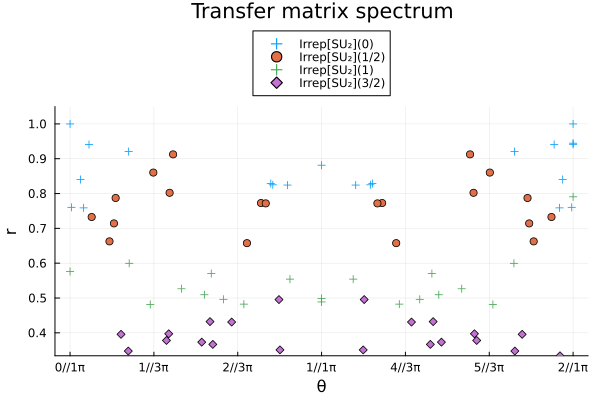

Nevertheless, using the symmetry, this can be remedied rather easily, by imposing the ground state to belong to a single class, and comparing the results. We can readily obtain 3 different criteria for determining the SPT phase of the ground state.

Firstly, we can compare variational energies for states of similar bond dimensions. As we expect the state of the wrong SPT phase to have to expend some of its expressiveness in correcting the SPT, it should have a harder time reaching lower energies.

Secondly, when inspecting the spectrum of the transfer matrix, we should see that the wrong SPT phase has a dominant value that is not in the trivial sector, which leads to a non-injective MPS.

Finally, the entanglement spectrum of the wrong SPT phase will show degeneracies of all singular values, which can again be attributed to an attempt to mimic the spectrum of the right SPT phase.

V_plus = SU2Space(0 => 10, 1 => 5, 2 => 3)
ψ_plus = InfiniteMPS(ℋ, V_plus)
ψ_plus, = find_groundstate(ψ_plus, H, VUMPS(; maxiter = 100))
E_plus = expectation_value(ψ_plus, H)

-1.4014193313393004 - 2.2233521403023605e-17im

V_minus = SU2Space(1 // 2 => 10, 3 // 2 => 5, 5 // 2 => 3)
ψ_minus = InfiniteMPS(ℋ, V_minus)
ψ_minus, = find_groundstate(ψ_minus, H, VUMPS(; maxiter = 100))
E_minus = expectation_value(ψ_minus, H)

-1.4014839739630827 + 6.744598315147384e-17im

transferp_plus = transferplot(
    ψ_plus;
    sectors = SU2Irrep[0, 1, 2], title = "ψ_plus", legend = :outertop
)
transferp_minus = transferplot(
    ψ_minus;
    sectors = SU2Irrep[0, 1, 2], title = "ψ_minus", legend = :outertop
)
plot(transferp_plus, transferp_minus; layout = (1, 2), size = (800, 400))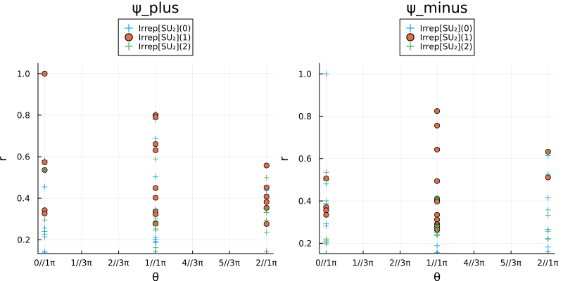

entanglementp_plus = entanglementplot(ψ_plus; title = "ψ_plus", legend = :outertop)
entanglementp_minus = entanglementplot(ψ_minus; title = "ψ_minus", legend = :outertop)
plot(entanglementp_plus, entanglementp_minus; layout = (1, 2), size = (800, 400))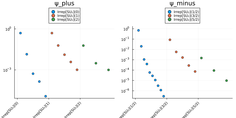

As we can see, the ground state can be found in the non-trivial SPT phase, 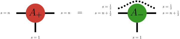. We can obtain an intuitive understanding of by considering the following diagram. If we denote the MPS tensors that make up the ground state as , we can construct a state in the trivial SPT phase that approximates the ground state as follows:

In other words, we can factorize a purely virtual isomorphism of   in order to obtain the ground state. This then also explains the degeneracies in the entanglement spectrum as well as in the transfer matrix spectrum. Finally, we can further confirm this intuition by looking at the entanglement entropy of the ground state. As we can see, the entanglement entropy of the state in the wrong SPT phase is exactly higher than the one in the right SPT phase, which is exactly what we would expect from the diagram above.

S_minus = sum(real, entropy(ψ_minus))
S_plus = sum(real, entropy(ψ_plus))
println("S_minus + log(2) = $(S_minus + log(2))")
println("S_plus = $S_plus")

S_minus + log(2) = 1.5486227235423025
S_plus = 1.545032353055433

---

This page was generated using Literate.jl.