A quantum quench

The previous tutorials computed ground states — static snapshots of a model at its lowest energy. This tutorial adds the time axis: we take a state that is not an eigenstate of its Hamiltonian and watch it evolve under the Schrödinger equation,

tracking one local observable as a function of time. The protocol we use is the simplest and most common one in the field, a global quench, and the workhorse algorithm is TDVP, the time-dependent variational principle, driven one step at a time through timestep.

We stay with the transverse-field Ising model from Your first ground state, so the model-building and ground-state steps below should look familiar.

Loading the packages

Every code block on this page shares one Julia session, so we load the packages once. As before, the model comes from MPSKitModels, the local spin operators from TensorKitTensors, and Plots draws the final figure.

using MPSKit, MPSKitModels, TensorKit
using TensorKitTensors.SpinOperators: σˣ, σᶻ
using Plots

1. Prepare the initial state

Time evolution needs a definite starting state, and the standard choice is the ground state of some Hamiltonian. We take a chain of L = 12 sites with a transverse field g₀ = 0.5 — the ordered side of the model — and find its ground state exactly as in the first tutorial, silencing the convergence log with verbosity = 0. The bond dimension D = 16 is comfortably large for a ground state of this size; we will see below why time evolution wants more headroom than a ground-state calculation.

L = 12
D = 16
g₀ = 0.5
H₀ = transverse_field_ising(FiniteChain(L); g = g₀)
ψ₀ = FiniteMPS(L, ℂ^2, ℂ^D)
ψ, = find_groundstate(ψ₀, H₀, DMRG(; verbosity = 0))

The observable we will track through the evolution is the transverse magnetization at the middle of the chain, away from the open ends. <!– REVIEW: I track ⟨σˣ⟩ rather than ⟨σᶻ⟩ because on a finite chain of this size the ground state respects the model's spin-flip symmetry, so ⟨σᶻ⟩ vanishes identically both before and after the quench and carries no dynamics to show; ⟨σˣ⟩ does not rely on symmetry breaking and is set directly by the transverse-field term. Please confirm this framing is the right one to give a reader. –> We measure its baseline value in the pre-quench ground state:

i_mid = L ÷ 2
real(expectation_value(ψ, i_mid => σˣ()))

0.259111670940287

2. The quench

A global quench is the sudden change of a parameter of the Hamiltonian, everywhere at once: we prepare the ground state of H₀, then at t = 0 switch the Hamiltonian to a different H₁ and let the state evolve under it. Because ψ is an eigenstate of H₀ but not of H₁, it is no longer stationary — the quench injects energy into the system, and nontrivial dynamics follows.

Our quench takes the transverse field from g₀ = 0.5 all the way across the phase transition to g₁ = 2.0:

g₁ = 2.0
H₁ = transverse_field_ising(FiniteChain(L); g = g₁)

12-site FiniteMPOHamiltonian(ComplexF64, TensorKit.ComplexSpace) with maximal dimension 3:
┬─[12]─ ℂ^2
│ (ℂ^1 ⊞ ℂ^1 ⊞ ℂ^1)
┼─[11]─ ℂ^2
│ (ℂ^1 ⊞ ℂ^1 ⊞ ℂ^1)
┼─[10]─ ℂ^2
│ (ℂ^1 ⊞ ℂ^1 ⊞ ℂ^1)
┼─[9]─ ℂ^2
│ (ℂ^1 ⊞ ℂ^1 ⊞ ℂ^1)
│ ⋮
│ (ℂ^1 ⊞ ℂ^1 ⊞ ℂ^1)
┼─[3]─ ℂ^2
│ (ℂ^1 ⊞ ℂ^1 ⊞ ℂ^1)
┼─[2]─ ℂ^2
│ (ℂ^1 ⊞ ℂ^1 ⊞ ℂ^1)
┴─[1]─ ℂ^2

<!– REVIEW: physics expectation for this quench — since H₁ sits deep in the disordered phase, I state below (Section 5) that the transverse magnetization relaxes towards a new value with oscillations. Please confirm this description of the post-quench dynamics. –>

3. A single time step

The elementary move of real-time evolution in MPSKit is timestep, which advances a state by one small increment dt. Its arguments are, in order: the state, the Hamiltonian to evolve under, the current time, the step size, and the algorithm. Here we take the very first step, from t = 0.0 to t = dt, with single-site TDVP:

dt = 0.05
ψ_t, envs = timestep(ψ, H₁, 0.0, dt, TDVP())
real(expectation_value(ψ_t, i_mid => σˣ()))

0.2734182381548043

TDVP integrates the Schrödinger equation projected onto the space of MPS with the current bond dimension, which is why it slots so naturally into an MPS workflow.

timestep returns two things:

• ψ_t — the evolved state at time dt (a new state; ψ is left untouched).

• envs — the environments, cached partial contractions belonging to the new state and H₁.

The envs are the reason evolution loops are cheap to keep running: passing them back into the next timestep call lets it start from the cached contractions instead of recomputing them from scratch.

The transverse magnetization has already moved slightly away from its t = 0 value — the state is on its way.

4. Evolving in a loop

Real-time evolution is nothing more than this single step, repeated. We already took step 1 above, so the loop below performs the remaining steps, up to n_steps = 40 in total (a final time of t = 2.0), recording the transverse magnetization at the middle of the chain after every step. Note how each iteration feeds the previous envs back in as the optional last argument, and how the current time (n - 1) * dt advances with the loop.

n_steps = 40
times = (0:n_steps) .* dt
m = zeros(n_steps + 1)
m[1] = real(expectation_value(ψ, i_mid => σˣ()))    # t = 0, before the quench dynamics
m[2] = real(expectation_value(ψ_t, i_mid => σˣ()))  # t = dt, from the single step above
for n in 2:n_steps
    global ψ_t, envs
    ψ_t, envs = timestep(ψ_t, H₁, (n - 1) * dt, dt, TDVP(), envs)
    m[n + 1] = real(expectation_value(ψ_t, i_mid => σˣ()))
end
m[end]

0.4876906440506108

(The global keyword is needed because the loop rebinds ψ_t and envs, which live outside it; inside a function you would not need it.)

Writing the loop by hand like this keeps every moving part visible, which is the point of a tutorial. For production use, time_evolve wraps exactly this loop and steps through a whole vector of time points in one call — see Time evolution.

5. Magnetization over time

The payoff: the transverse magnetization at the middle of the chain, as a function of time after the quench.

plot(times, m;
    xlabel = "t", ylabel = "⟨σˣ⟩ at site $i_mid",
    label = "TDVP, D = $D", title = "TFIM transverse magnetization after a quench")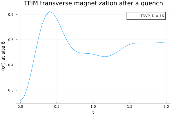

The curve shows how the observable responds to the sudden change in the field: starting from its pre-quench value, relaxes towards a new value set by H₁, with oscillations along the way. <!– REVIEW: same physics claim as flagged in Section 2 — relaxation towards a new value with oscillations for this g = 0.5 → 2.0 quench at L = 12; please verify against the actual curve the build produces. –>

Fixed bond dimension means finite reach in time

Single-site TDVP keeps the bond dimension fixed at whatever the initial state has. After a quench, however, the entanglement of the evolving state grows with time, so a fixed bond dimension can only follow the true dynamics faithfully up to some finite time — beyond it, the simulation quietly loses accuracy rather than failing loudly. <!– REVIEW: entanglement growth after a global quench (often stated as linear growth) and the resulting finite time window at fixed bond dimension — please confirm this framing. –> The practical checks and remedies — two-site TDVP2, which grows the bond dimension as it truncates, and bond-expansion options for single-site TDVP — are collected in Time evolution.

Where to go next

You have run your first dynamics simulation: prepare a ground state, quench the Hamiltonian, step the state forward in time, and read off an observable at every step.

The natural reference for everything this page glossed over is the Time evolution how-to: evolving over a time span in one call, growing the bond dimension during evolution, imaginary time, and evolving infinite states. Speaking of which — everything here was done on a finite chain, but timestep works just as well on the InfiniteMPS states introduced in The thermodynamic limit. And for measuring more than a single local magnetization on the evolved states, see Computing observables.