The Ising CFT spectrum

This tutorial is meant to show the finite size CFT spectrum for the quantum Ising model. We do this by first employing an exact diagonalization technique, and then extending the analysis to larger system sizes through the use of MPS techniques.

using MPSKit, MPSKitModels, TensorKit, Plots, KrylovKit
using LinearAlgebra: eigvals, diagm, Hermitian

The Hamiltonian is defined on a finite lattice with periodic boundary conditions, which can be implemented as follows:

L = 12
H = periodic_boundary_conditions(transverse_field_ising(), L)

12-site FiniteMPOHamiltonian(ComplexF64, TensorKit.ComplexSpace) with maximal dimension 6:
┬─[12]─ ℂ^2
│ (ℂ^1 ⊞ ℂ^1 ⊞ ℂ^1 ⊞ ⋯ ⊞ ℂ^1 ⊞ ℂ^1 ⊞ ℂ^1)
┼─[11]─ ℂ^2
│ (ℂ^1 ⊞ ℂ^1 ⊞ ℂ^1 ⊞ ⋯ ⊞ ℂ^1 ⊞ ℂ^1 ⊞ ℂ^1)
┼─[10]─ ℂ^2
│ (ℂ^1 ⊞ ℂ^1 ⊞ ℂ^1 ⊞ ⋯ ⊞ ℂ^1 ⊞ ℂ^1 ⊞ ℂ^1)
┼─[9]─ ℂ^2
│ (ℂ^1 ⊞ ℂ^1 ⊞ ℂ^1 ⊞ ⋯ ⊞ ℂ^1 ⊞ ℂ^1 ⊞ ℂ^1)
│ ⋮
│ (ℂ^1 ⊞ ℂ^1 ⊞ ℂ^1 ⊞ ⋯ ⊞ ℂ^1 ⊞ ℂ^1 ⊞ ℂ^1)
┼─[3]─ ℂ^2
│ (ℂ^1 ⊞ ℂ^1 ⊞ ℂ^1 ⊞ ⋯ ⊞ ℂ^1 ⊞ ℂ^1 ⊞ ℂ^1)
┼─[2]─ ℂ^2
│ (ℂ^1 ⊞ ℂ^1 ⊞ ℂ^1 ⊞ ⋯ ⊞ ℂ^1 ⊞ ℂ^1 ⊞ ℂ^1)
┴─[1]─ ℂ^2

Exact diagonalisation

In MPSKit, there is support for exact diagonalisation by leveraging the fact that applying the Hamiltonian to an untruncated MPS will result in an effective Hamiltonian on the center site which implements the action of the entire Hamiltonian. Thus, optimizing the middle tensor is equivalent to optimixing a state in the entire Hilbert space, as all other tensors are just unitary matrices that mix the basis.

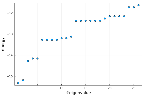
energies, states = exact_diagonalization(H; num = 18, alg = Lanczos(; krylovdim = 200));
plot(
    real.(energies);
    seriestype = :scatter, legend = false, ylabel = "energy", xlabel = "#eigenvalue"
)

Krylov dimension

Note that we have specified a large Krylov dimension as degenerate eigenvalues are notoriously difficult for iterative methods.

Extracting momentum

Given a state, it is possible to assign a momentum label through the use of the translation operator. This operator can be defined in MPO language either diagramatically as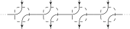

or in the code as:

function O_shift(L)
    I = id(ComplexF64, ℂ^2)
    @tensor O[W S; N E] := I[W; N] * I[S; E]
    return periodic_boundary_conditions(InfiniteMPO([O]), L)
end

O_shift (generic function with 1 method)

We can then calculate the momentum of the ground state as the expectation value of this operator. However, there is a subtlety because of the degeneracies in the energy eigenvalues. The eigensolver will find an orthonormal basis within each energy subspace, but this basis is not necessarily a basis of eigenstates of the translation operator. In order to fix this, we diagonalize the translation operator within each energy subspace. The resulting energy levels have one-to-one correspondence to the operators in CFT, where the momentum is related to their conformal spin as  .

function fix_degeneracies(basis)
    L = length(basis[1])
    M = zeros(ComplexF64, length(basis), length(basis))
    T = O_shift(L)
    for j in eachindex(basis), i in eachindex(basis)
        M[i, j] = dot(basis[i], T, basis[j])
    end

    vals = eigvals(M)
    return angle.(vals)
end

momenta = Float64[]
append!(momenta, fix_degeneracies(states[1:1]))
append!(momenta, fix_degeneracies(states[2:2]))
append!(momenta, fix_degeneracies(states[3:3]))
append!(momenta, fix_degeneracies(states[4:5]))
append!(momenta, fix_degeneracies(states[6:9]))
append!(momenta, fix_degeneracies(states[10:11]))
append!(momenta, fix_degeneracies(states[12:12]))
append!(momenta, fix_degeneracies(states[13:16]))
append!(momenta, fix_degeneracies(states[17:18]))

18-element Vector{Float64}:
 -6.835457747908734e-17
 -1.5823223400041525e-17
 -2.117254204162227e-17
 -0.5235987755982994
  0.5235987755982988
 -1.047197551196598
  1.0471975511965976
  0.5235987755982993
 -0.5235987755982985
 -1.0471975511965976
  1.0471975511965976
 -1.3705449793358471e-17
  1.570796326794897
 -1.5707963267948966
 -1.0471975511965979
  1.0471975511965976
  1.5707963267948968
 -1.5707963267948966

We can compute the scaling dimensions of the operators in the CFT from the energy gap of the corresponding excitations as   , where  . If we plot these scaling dimensions against the conformal spin from above, we retrieve the familiar spectrum of the Ising CFT.

v = 2.0
Δ = real.(energies[1:18] .- energies[1]) ./ (2π * v / L)
S = momenta ./ (2π / L)

p = plot(
    S, real.(Δ);
    seriestype = :scatter, xlabel = "conformal spin (S)", ylabel = "scaling dimension (Δ)",
    legend = false
)
vline!(p, -3:3; color = "gray", linestyle = :dash)
hline!(p, [0, 1 / 8, 1, 9 / 8, 2, 17 / 8]; color = "gray", linestyle = :dash)
p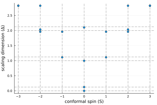

Finite bond dimension

If we limit the maximum bond dimension of the MPS, we get an approximate solution, but we can reach higher system sizes.

L_mps = 20
H_mps = periodic_boundary_conditions(transverse_field_ising(), L_mps)
D = 64
ψ, envs, δ = find_groundstate(FiniteMPS(L_mps, ℂ^2, ℂ^D), H_mps, DMRG(; verbosity = 0));

Excitations on top of the ground state can be found through the use of the quasiparticle ansatz. This returns quasiparticle states, which can be converted to regular FiniteMPS objects.

E_ex, qps = excitations(H_mps, QuasiparticleAnsatz(), ψ, envs; num = 18)
states_mps = vcat(ψ, map(qp -> convert(FiniteMPS, qp), qps))
energies_mps = map(x -> expectation_value(x, H_mps), states_mps)

momenta_mps = Float64[]
append!(momenta_mps, fix_degeneracies(states_mps[1:1]))
append!(momenta_mps, fix_degeneracies(states_mps[2:2]))
append!(momenta_mps, fix_degeneracies(states_mps[3:3]))
append!(momenta_mps, fix_degeneracies(states_mps[4:5]))
append!(momenta_mps, fix_degeneracies(states_mps[6:9]))
append!(momenta_mps, fix_degeneracies(states_mps[10:11]))
append!(momenta_mps, fix_degeneracies(states_mps[12:12]))
append!(momenta_mps, fix_degeneracies(states_mps[13:16]))
append!(momenta_mps, fix_degeneracies(states_mps[17:18]))

v = 2.0
Δ_mps = real.(energies_mps[1:18] .- energies_mps[1]) ./ (2π * v / L_mps)
S_mps = momenta_mps ./ (2π / L_mps)

p_mps = plot(
    S_mps, real.(Δ_mps);
    seriestype = :scatter, xlabel = "conformal spin (S)",
    ylabel = "scaling dimension (Δ)", legend = false
)
vline!(p_mps, -3:3; color = "gray", linestyle = :dash)
hline!(p_mps, [0, 1 / 8, 1, 9 / 8, 2, 17 / 8]; color = "gray", linestyle = :dash)
p_mps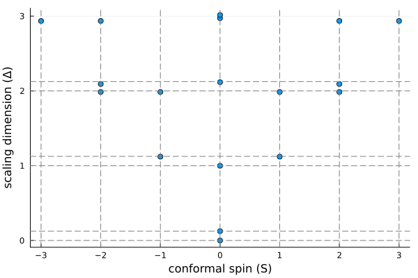

---

This page was generated using Literate.jl.