MPSKit.jlMatrix product states in Julia

MPSKit.jl simulates one-dimensional quantum many-body systems with matrix product states and operators, at finite size or directly in the thermodynamic limit. Built on the TensorKit.jl tensor backend, it is aimed at researchers and students who want tensor-network calculations without reimplementing the underlying machinery.

Installation ​

MPSKit.jl is a part of the general registry. Together with the packages used throughout this documentation, it can be installed via the package manager as:

pkg> add MPSKit TensorKit MPSKitModels TensorKitTensors Plots

• MPSKit provides the matrix product state and operator types, together with the ground-state, time-evolution, and bond-dimension algorithms.

• TensorKit supplies the tensor backend (TensorMaps and vector spaces) that MPSKit is built on; it also re-exports the @tensor macro for contracting tensors by hand, along with truncation-scheme constructors such as truncrank (from MatrixAlgebraKit).

• MPSKitModels collects pre-defined Hamiltonians and local operators for common physical models.

• TensorKitTensors provides ready-made local operators, such as the Pauli operators used throughout the documentation.

• Plots is used to visualize results in several of the how-to guides and examples.

For a step-by-step walkthrough that sets up a dedicated environment and verifies the installation, see Installation.

A first calculation ​

Almost every MPSKit calculation follows the same three steps: build a Hamiltonian, optimize a state, and read off observables. The transverse-field Ising chain (TFIM) makes each step concrete in a few lines.

1. Build a Hamiltonian ​

MPO Hamiltonians are assembled directly from local operators, so an arbitrary model — not just the built-in ones — takes only a couple of lines. Here the single-site Pauli operators come from TensorKitTensors, and the TFIM is a nearest-neighbour σᶻσᶻ coupling plus a transverse σˣ field:

using MPSKit, TensorKit
using TensorKitTensors.SpinOperators: σˣ, σᶻ

L = 16
g = 0.5
lattice = fill(ℂ^2, L)
H = FiniteMPOHamiltonian(lattice, (i, i + 1) => -(σᶻ() ⊗ σᶻ()) for i in 1:(L - 1)) +
    FiniteMPOHamiltonian(lattice, (i,) => -g * σˣ() for i in 1:L)

16-site FiniteMPOHamiltonian(ComplexF64, TensorKit.ComplexSpace) with maximal dimension 3:
┬─[16]─ ℂ^2
│ (ℂ^1 ⊞ ℂ^1 ⊞ ℂ^1)
┼─[15]─ ℂ^2
│ (ℂ^1 ⊞ ℂ^1 ⊞ ℂ^1)
┼─[14]─ ℂ^2
│ (ℂ^1 ⊞ ℂ^1 ⊞ ℂ^1)
┼─[13]─ ℂ^2
│ (ℂ^1 ⊞ ℂ^1 ⊞ ℂ^1)
│ ⋮
│ (ℂ^1 ⊞ ℂ^1 ⊞ ℂ^1)
┼─[3]─ ℂ^2
│ (ℂ^1 ⊞ ℂ^1 ⊞ ℂ^1)
┼─[2]─ ℂ^2
│ (ℂ^1 ⊞ ℂ^1 ⊞ ℂ^1)
┴─[1]─ ℂ^2

See Building Hamiltonians for infinite lattices, longer-range terms, and boundary conditions.

2. Optimize a state ​

Start from an initial FiniteMPS of bond dimension 16 and pass it, together with the Hamiltonian, to find_groundstate. The algorithm — here DMRG — is an ordinary argument, and its keywords (tolerance, iteration count, verbosity) tune the optimization:

ψ₀ = FiniteMPS(L, ℂ^2, ℂ^16)
ψ, envs, ϵ = find_groundstate(ψ₀, H, DMRG(; tol = 1e-10, verbosity = 0))
ϵ   # final convergence error

7.268170737343598e-11

Choosing a different optimizer such as VUMPS, or raising the bond dimension, is a one-line change; see Ground-state algorithms.

3. Read off observables ​

Expectation values are a single call. The ground-state energy is just the Hamiltonian evaluated on the state:

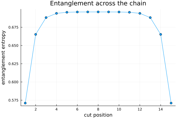
E = expectation_value(ψ, H)

-16.146050955496793 - 4.321906294290561e-15im

Local operators, correlators, and entanglement measures work the same way. For instance, the von Neumann entropy across each bond traces out the entanglement profile of the chain:

using Plots
S = [real(entropy(ψ, i)) for i in 1:(L - 1)]
plot(
    1:(L - 1), S; xlabel = "cut position", ylabel = "entanglement entropy",
    marker = :circle, legend = false, title = "Entanglement across the chain"
)

See Computing observables and Entanglement entropy and spectrum for the full set, and Your first ground state for a guided walkthrough of this calculation.

Beyond this example ​

The same three steps carry over to harder problems, usually by changing only the vector spaces or the state type:

• The thermodynamic limit works at infinite system size: replace FiniteMPS with an InfiniteMPS and DMRG with VUMPS, and the rest of the code is unchanged.

• Using symmetries imposes abelian or non-abelian symmetries by swapping the plain ℂ^2 spaces for symmetric ones (for example an SU2Space), which also shrinks the bond dimension; see also the Haldane gap example.

• The Hubbard model treats fermions with the same machinery, through TensorKit's graded vector spaces.

Where next ​

• Installation and Your first ground state open the tutorial track, walking through complete calculations from scratch.

• How-to guides are focused recipes for a known task, such as constructing states, building Hamiltonians, and computing observables.

• The manual explains the concepts behind the library, including States, Operators, and Algorithms.

• The examples gallery collects longer, fully worked case studies across symmetries, infinite systems, and less common algorithms.

• The public API is the curated, stable entry point to the full library reference.

Ecosystem ​

MPSKit builds on TensorKit.jl, which supplies the tensors and vector spaces and handles the symmetries. Models and ready-made operators come from MPSKitModels.jl and TensorKitTensors.jl. All of these are part of the QuantumKitHub organization; the TensorKit documentation is available here.

Community and support ​

Questions and general discussion are welcome on GitHub Discussions; bug reports belong on the issue tracker. If you would like to contribute, see CONTRIBUTING.md on GitHub.

Citing MPSKit ​

If MPSKit.jl is useful for your research, please consider citing it — a citation is the most direct way to support the project and helps others find it. The package is archived on Zenodo under the DOI 10.5281/zenodo.10654900. The CITATION.cff file in the repository always holds the up-to-date metadata, or you can use the BibTeX entry below:

@software{mpskitjl,
  author  = {Devos, Lukas and Van Damme, Maarten and Haegeman, Jutho},
  title   = {{MPSKit.jl}},
  version = {v0.13.13},
  doi     = {10.5281/zenodo.10654900},
  url     = {https://github.com/QuantumKitHub/MPSKit.jl},
  year    = {2026}
}