



The Haldane gap
In this tutorial we will calculate the Haldane gap (the energy gap in the
using MPSKit, MPSKitModels, TensorKit, Plots, PolynomialsThe Heisenberg model is defined by the following Hamiltonian:
This Hamiltonian has an SU(2) symmetry, which we can enforce by using SU(2)-symmetric tensors:
symmetry = SU2Irrep
spin = 1
J = 11Finite size extrapolation
We can start the analysis using finite-size methods. The ground state of this model can be approximated using finite MPS through the use of DMRG.
The typical way to find excited states is to minimize the energy while adding an error term
In Steven White's original DMRG paper it was remarked that the
L = 11
chain = FiniteChain(L)
H = heisenberg_XXX(symmetry, chain; J, spin)

physical_space = SU2Space(1 => 1)
virtual_space = SU2Space(0 => 12, 1 => 12, 2 => 5, 3 => 3)
ψ₀ = FiniteMPS(L, physical_space, virtual_space)
ψ, envs, delta = find_groundstate(ψ₀, H, DMRG(; verbosity = 0))
E₀ = real(expectation_value(ψ, H))
En_1, st_1 = excitations(H, QuasiparticleAnsatz(), ψ, envs; sector = SU2Irrep(1))
En_2, st_2 = excitations(H, QuasiparticleAnsatz(), ψ, envs; sector = SU2Irrep(2))
ΔE_finite = real(En_2[1] - En_1[1])0.7989253589480472We can go even further and doublecheck the claim that
p_density = plot(; xaxis = "position", yaxis = "energy density")
excited_1 = convert(FiniteMPS, st_1[1])
excited_2 = convert(FiniteMPS, st_2[1])
SS = -S_exchange(ComplexF64, SU2Irrep; spin = 1)
e₀ = [real(expectation_value(ψ, (i, i + 1) => SS)) for i in 1:(L - 1)]
e₁ = [real(expectation_value(excited_1, (i, i + 1) => SS)) for i in 1:(L - 1)]
e₂ = [real(expectation_value(excited_2, (i, i + 1) => SS)) for i in 1:(L - 1)]
plot!(p_density, e₀; label = "S = 0")
plot!(p_density, e₁; label = "S = 1")
plot!(p_density, e₂; label = "S = 2")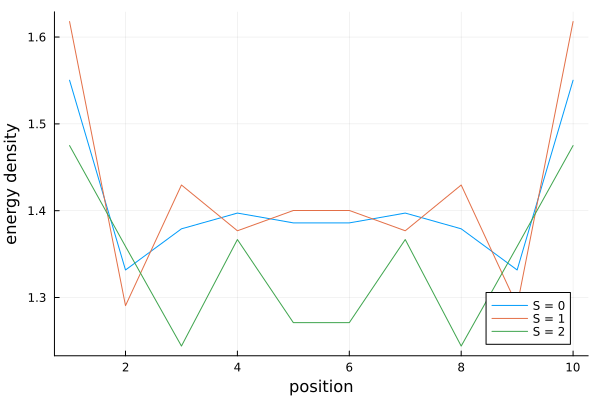
Finally, we can obtain a value for the Haldane gap by extrapolating our results for different system sizes.
Ls = 12:4:30
ΔEs = map(Ls) do L
    @info "computing L = $L"
    ψ₀ = FiniteMPS(L, physical_space, virtual_space)
    H = heisenberg_XXX(symmetry, FiniteChain(L); J, spin)
    ψ, envs, delta = find_groundstate(ψ₀, H, DMRG(; verbosity = 0))
    En_1, st_1 = excitations(H, QuasiparticleAnsatz(), ψ, envs; sector = SU2Irrep(1))
    En_2, st_2 = excitations(H, QuasiparticleAnsatz(), ψ, envs; sector = SU2Irrep(2))
    return real(En_2[1] - En_1[1])
end

f = fit(Ls .^ (-2), ΔEs, 1)
ΔE_extrapolated = f.coeffs[1]0.4517340158583749p_size_extrapolation = plot(; xaxis = "L^(-2)", yaxis = "ΔE", xlims = (0, 0.015))
plot!(p_size_extrapolation, Ls .^ (-2), ΔEs; seriestype = :scatter, label = "numerical")
plot!(p_size_extrapolation, x -> f(x); label = "fit")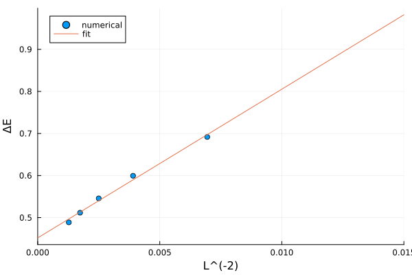
Thermodynamic limit
A much nicer way of obtaining the Haldane gap is by working directly in the thermodynamic limit. As was already hinted at by the edge modes, this model is in a non-trivial SPT phase. Thus, care must be taken when selecting the symmetry sectors. The ground state has half-integer edge modes, thus the virtual spaces must also all carry half-integer charges.
In contrast with the finite size case, we now should specify a momentum label to the excitations. This way, it is possible to scan the dispersion relation over the entire momentum space.
chain = InfiniteChain(1)
H = heisenberg_XXX(symmetry, chain; J, spin)
virtual_space_inf = Rep[SU₂](1 // 2 => 16, 3 // 2 => 16, 5 // 2 => 8, 7 // 2 => 4)
ψ₀_inf = InfiniteMPS([physical_space], [virtual_space_inf])
ψ_inf, envs_inf, delta_inf = find_groundstate(ψ₀_inf, H; verbosity = 0)

kspace = range(0, π, 16)
Es, _ = excitations(H, QuasiparticleAnsatz(), kspace, ψ_inf, envs_inf; sector = SU2Irrep(1))

ΔE, idx = findmin(real.(Es))
println("minimum @k = $(kspace[idx]):\t ΔE = $(ΔE)")
[ Info: Found excitations for momentum = 0.0
[ Info: Found excitations for momentum = 0.20943951023931953
[ Info: Found excitations for momentum = 0.41887902047863906
[ Info: Found excitations for momentum = 0.6283185307179586
[ Info: Found excitations for momentum = 1.4660765716752369
[ Info: Found excitations for momentum = 1.2566370614359172
[ Info: Found excitations for momentum = 0.8377580409572781
[ Info: Found excitations for momentum = 1.0471975511965976
[ Info: Found excitations for momentum = 1.6755160819145563
[ Info: Found excitations for momentum = 1.8849555921538759
[ Info: Found excitations for momentum = 2.0943951023931953
[ Info: Found excitations for momentum = 2.303834612632515
[ Info: Found excitations for momentum = 2.5132741228718345
[ Info: Found excitations for momentum = 2.9321531433504737
[ Info: Found excitations for momentum = 2.722713633111154
[ Info: Found excitations for momentum = 3.141592653589793
minimum @k = 3.141592653589793: ΔE = 0.41047924848831047plot(kspace, real.(Es); xaxis = "momentum", yaxis = "ΔE", label = "S = 1")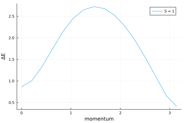
This page was generated using Literate.jl.