The SU(3) Heisenberg chain

The spin-1 Heisenberg chain famously has a gapped, symmetry-protected topological ground state: the Haldane phase. A natural question is what happens when the symmetry of the spins is promoted to a larger symmetry. In this example we study the generalization introduced in (Devos et al., 2022): a uniform chain where every site carries the fully-symmetric    irrep of (the ten-dimensional representation), coupled by a nearest-neighbour -invariant Heisenberg interaction

where the are the eight generators of . This is the direct analog of the spin-1 chain, with the three generators of replaced by the eight generators of . The goal of this example is to exercise the full toolchain end to end — building the symmetric Hamiltonian, optimizing a uniform ground state with VUMPS, and scanning an excitation dispersion — rather than to pin down the model's (very small) gap to high accuracy; we return to that point in the closing discussion.

Working with the full non-abelian symmetry is what makes this tractable. Just as symmetry drastically shrinks the spin-1 problem (see Symmetries), imposing block-diagonalizes every tensor along its irreducible representations, so that a modest number of variational parameters already captures a large physical bond dimension. The Clebsch–Gordan coefficients that this requires are provided by SUNRepresentations.jl, whose SU3Irrep sectors plug directly into TensorKit's graded vector spaces.

First-run cost

SUNRepresentations.jl computes Clebsch–Gordan coefficients on demand and caches them both in memory and on disk (via Scratch.jl). The first time a given coefficient is needed the computation can be slow; later runs reuse the on-disk cache. On a machine without a persisted scratch cache — such as a fresh continuous-integration runner — this example therefore pays the full coefficient-generation cost once.

using TensorKit
using SUNRepresentations
using MPSKit
using Plots

For reproducibility of this page, we fix the seed of the random number generator:

using Random
Random.seed!(4321);

The model

Each site carries the    irrep, which we obtain from its highest weight and represent as a one-dimensional graded space.

I300 = SU3Irrep(3, 0, 0)
Vphys = Vect[SU3Irrep](I300 => 1)
@show dim(I300)

10

To build the interaction we use the same Casimir trick as for the chain. Writing   for the quadratic Casimir operator, the two-site coupling is diagonal in the total charge of a bond:

SUNRepresentations.jl provides the quadratic Casimir through casimir(2, irrep). Its normalization is the standard one with  : the fundamental    has    .

@show casimir(2, SU3Irrep(1, 0, 0))
@show casimir(2, I300)

6//1

The nearest-neighbour term is then a single TensorKit operator that acts as a scalar on each fusion channel of      . Constructing it by iterating over the blocks — one block per total charge — mirrors the construction, but now with casimir(2, ⋅) supplying the eigenvalues.

function su3_heisenberg(Vphys; J = 1.0)
    site = SU3Irrep(3, 0, 0)
    c2_site = casimir(2, site)
    SS = zeros(ComplexF64, Vphys ⊗ Vphys ← Vphys ⊗ Vphys)
    for (c, data) in blocks(SS)
        coupling = (casimir(2, c) - 2 * c2_site) / 2
        for i in axes(data, 1)
            data[i, i] = J * coupling
        end
    end
    return InfiniteMPOHamiltonian(SS)
end

H = su3_heisenberg(Vphys)

1-site InfiniteMPOHamiltonian(ComplexF64, Rep[SU₃]) with maximal dimension 10:
| ⋮
| (((0, 0, 0)=>1) ⊞ ((2, 1, 0)=>1) ⊞ ((0, 0, 0)=>1))
┼─[1]─ ((3, 0, 0) => 1)
│ (((0, 0, 0)=>1) ⊞ ((2, 1, 0)=>1) ⊞ ((0, 0, 0)=>1))
| ⋮

We can read off the physics directly from the fusion channels. The product       decomposes into four irreps, and the antiferromagnetic coupling ( ) favours the channels of lowest Casimir:

for (c, n) in directproduct(I300, I300)
    coupling = (casimir(2, c) - 2 * casimir(2, I300)) / 2
    println(rpad(string(c), 22), " dim = ", rpad(dim(c), 4), " coupling = ", coupling)
end

Irrep[SU₃]((6, 0, 0))  dim = 28   coupling = 3//1
Irrep[SU₃]((5, 1, 0))  dim = 35   coupling = 0//1
Irrep[SU₃]((4, 2, 0))  dim = 27   coupling = -2//1
Irrep[SU₃]((3, 3, 0))  dim = 10   coupling = -3//1

Ground state

The    irrep has trivial triality (congruency class ), so — like the integer-spin Haldane chain — a translation-invariant state on a single-site unit cell is admissible. Because the physical charge has triality it cannot shift the triality of the virtual bonds, so every virtual space must sit in a single congruency class; here we use the trivial class , which we found to give the lowest variational energy. Following (Devos et al., 2022), we seed the optimization with a random -symmetric uniform state and optimize with VUMPS. The bond dimension is kept deliberately modest here so that the page builds quickly.

Vvirt = Vect[SU3Irrep](
    SU3Irrep(0, 0, 0) => 8,
    SU3Irrep(2, 1, 0) => 6,
    SU3Irrep(3, 0, 0) => 3,
    SU3Irrep(3, 3, 0) => 3,
    SU3Irrep(4, 2, 0) => 2,
)
@show dim(Vvirt)

ψ₀ = InfiniteMPS([Vphys], [Vvirt])
ψ, envs, δ = find_groundstate(ψ₀, H, VUMPS(; maxiter = 200, tol = 1.0e-10, verbosity = 1))
E₀ = real(expectation_value(ψ, H))
println("ground-state energy per site: E₀ = $E₀")

dim(Vvirt) = 170
┌ Warning: Constructing an MPS from tensors that are not full rank
└ @ MPSKit ~/Projects/MPSKit.jl/docs/src/states/infinitemps.jl:180
ground-state energy per site: E₀ = -2.573505652431292

The excitation spectrum

On top of the ground state we compute excitations with the quasiparticle ansatz. In the thermodynamic limit each excitation carries a definite momentum and a definite charge. Following (Devos et al., 2022), we look in the adjoint    sector, where that reference finds the lowest branch, and scan across half of the Brillouin zone (the other half follows by reflection).

sector = SU3Irrep(2, 1, 0)
kspace = range(0, π, 10)
Es, _ = excitations(H, QuasiparticleAnsatz(), kspace, ψ, envs; sector)

Δ, idx = findmin(real.(Es))
println("branch minimum ΔE/J = $Δ at k = $(kspace[idx])")

branch minimum ΔE/J = -0.041856660250392086 at k = 2.0943951023931953

plot(
    kspace, real.(Es);
    xaxis = "momentum k", yaxis = "ΔE / J", label = "[2 1 0] branch",
    title = "SU(3) [3 0 0] excitation dispersion"
)
hline!([0.0]; color = :gray, linestyle = :dash, label = "")
vline!([2π / 3]; color = :gray, linestyle = :dot, label = "k = 2π/3")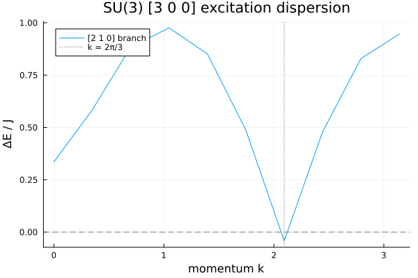

The branch has a pronounced soft mode at  , exactly the momentum at which (Devos et al., 2022) locates the minimum of the dispersion, where that reference reports a gap of  .

The soft-mode location is reproduced cleanly, but the gap value is not, and it is worth being precise about why. The quasiparticle energies plotted above are a genuine variational upper bound on the excitation energies only when they are measured relative to the exact ground state. Here the ground state is a deliberately lightweight, modest-bond-dimension uniform MPS, and for this near-critical model it is not converged to that accuracy. Because the reference state sits slightly too high in energy, the ansatz can find "excitations" that lie below it, so near   the computed branch drops to essentially zero and even slightly negative. The dispersion here is therefore not a variational estimate of the true gap: the small value   is quoted from (Devos et al., 2022) and would require a carefully converged, large-bond-dimension calculation to reproduce. What this example does show is the complete -symmetric workflow — Hamiltonian construction, VUMPS ground state, and a momentum-resolved excitation scan — with the soft mode correctly located at  .

---

This page was generated using Literate.jl.